
Introduction to R
Installing R and R Studio
R Studio is an excellent IDE (integrated development environment) for the R language which provides a variety of tools and quality of life features.
To get set up using R with R Studio, you should first install native R. Navigate here: https://cran.r-project.org/ and follow the links to the version of R that is compatible with your operating system. Once you’ve installed R you should then install R Studio, again paying attention to your particular operating system, by navigating here: https://www.rstudio.com/products/rstudio/download2/. For use on a single machine, choose the Desktop edition.
Working in R Studio: Always Send Commands from a Script
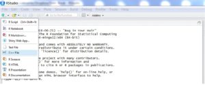
Once you open R studio, you’ll want to create a new R script from the file menu:
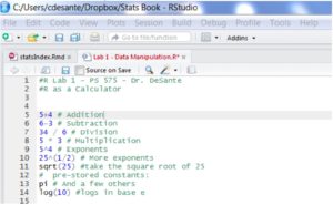
Once you type a few lines of code into the new script, it may look something like this:
To run or execute the code, simply click on a line (or highlight the portion of code you’d want to send) and either key ctrl + r (Windows) or cmd + enter (Mac OS). Once executed, the code will produce results in the console shown below:
> my.dice.simulator(10)
[1] 9.5
> my.dice.simulator(100)
[1] 10.53
> my.dice.simulator(1000)
[1] 10.473
> my.dice.simulator(5000)
[1] 10.4862
>
Setting a Working Directory
A working directory is the place where R looks for any files you’d like to load and saves any output or graphics. I’d advise using designated subfolders for each project.
Notice the direction of the slashes, as they vary between Mac and PC. The getwd() command will print the name of the folder you’ve specified so you can confirm you’ve done things correctly. Having a specified folder to save things to is especially nice when saving graphics, plots, etc.
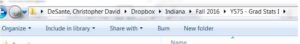
The folder shown above can be set as my working directory by using the following command:
getwd() #shows you your current working directory

> [1] "C:/Users/cdesante/Dropbox/Stats Book"

setwd( "C:/Users/cdesante/Dropbox/Indiana/Fall 2016/Y575 - Grad Stats I/" )
# Notice which way the / go; if you copy from Windows Explorer, you'll have to reverse them.
getwd() #Hey, look, we changed it!

> [1] "C:/Users/cdesante/Dropbox/Stats Book"
Alternatively, when working in R Studio, you could click on “Session” -> “Set Working Directory” -> “Choose Directory…” and navigate to the folder you would like to set as the working directory.
Assigning Object Names
Objects are things that reside in R’s workspace. There are three main rules for naming them:
1. EvErYThInG in R is CaSe SeNsITiVe
2. Object names cannot begin with a number
3. Object names cannot contain spaces.
Basic Coding Tips
As you first begin to code, everything is going to seem daunting, but there are a few things that you can do to make things easier for yourself:
1. Annotate your code so that someone else who reads it understands what you’re doing
2. Object names should be somewhat intuitive; if you wanted to name an object that contained a set of test scores you might name it “test.scores” as opposed to “ts2016” or “obj1,” etc.
3. Again, Object names cannot begin with a number, and they cannot contain spaces.
R as a Calculator
Now you know that code is written in the script window, processed by R, and then the results are shown in the Console window. From here on out this document will use embedded R code with the console output shown following the commands. For example, the next section shows the same code from above but with each block of code immediately followed by the R output it would generate. The lines of output begin with >. The [1] that begins each output line indicates the output has exactly one element. Chunks of code that all appear together can be thought of as being ‘sent’ to R in one command. You should also note that R is case sensitive; meaning that UPPER CASE and lower case letters will be interpreted differently.
5+4 # Addition
6-3 # Subtraction
34/6 # Division
5*3 # Multiplication
5^4 # Exponents
25^(1/2) # More exponents
sqrt(25) # take the square root of 25
# Pre-stored constants:
pi # And a few others
log(10) #logs in base e
> [1] 9
> [1] 3
> [1] 5.666667
> [1] 15
> [1] 625
> [1] 5
> [1] 5
> [1] 3.141593
> [1] 2.302585
You may notice that there are lines in this code that begin with #; these are comments left by the coder for anyone who may read the code at a later date. When R processes lines that begin with a # it ignores what is written after it until a new line begins.
NA # Missing value
NULL # Nothing
0/0 # NaN means "Not a number"
1/0 # Inf means infinity
# R also handles order of operations:
# Please Excuse My Dear Aunt Sally
2*(3-4)+2
2*(3-4)+2*(4+3)^(1/3)
exp(2) # e to the 2
> [1] NA
> NULL
> [1] NaN
> [1] Inf
> [1] 0
> [1] 1.825862
> [1] 7.389056